Machine Learning and Data Analytics in Petroleum Reservoir Engineering

Data-Driven Rate Optimization Under Geologic Uncertainty

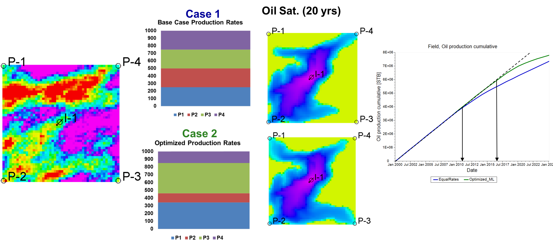
The most crucial decisions while operating an oilfield pertain to

a. At what rate should an operator extract oil from producer wells

b. At what rate should water be injected into the reservoir to push out maximum oil from the producer wells in (a.)

c. When/Where/Whether to drill the next well

The answers to all these questions are fairly elusive to the reservoir engineer owing not only to the uncertainty in the subsurface geology, but also a range on operational constraints that are required for safe operation. Moreover, in order to account for all the uncertain variables and constraints, one has to run a computationally-costly simulation a gazillion times.

My primary research focuses on solving some of these problems by invoking machine-learning at the simulation step. Specifically, I try to predict some aspects of the subsurface flow pattern, without having to run the costly simulation. It turns out that the machine-learning model runs faster than the simulation by around 3 orders of magnitude; so accounting for multiple variables, scenarios etc. becomes a breeze.

The first part of the work was presented at SPE-ATCE.

Using RNNs to Understand Reservoir Connectivity

In case we do not have a geologic model on which we can run the simulator, but have access to a lot of historical data (rates and pressures at operational wells in the field), we can use machine-learning based approaches to understand certain key aspects of the reservoir. One way to do this is to fit a recurrent neural net to the history and study the variable importance of each input (in this case, the injection rates) to each output (the production rates). However, the feasibility of such an approach is debated due to a number of reasons:

a. This approach needs historical data that ideally covers the entire space of possible inputs and underlying physics. This tends to be a major problem in reservoir engineering, wherein we have hundreds of wells, yet only a few years of data.

b. The RNN architecture and training (loss function formulation, window selection etc.) has to capture complex non-linear relationship between input and output. This problem is compounded by the fact that the underlying physics is generally not time-invariant. However, the approach is still worth a shot, given we have sufficient data and the physical regime does not change too much in the space where we make the predictions.

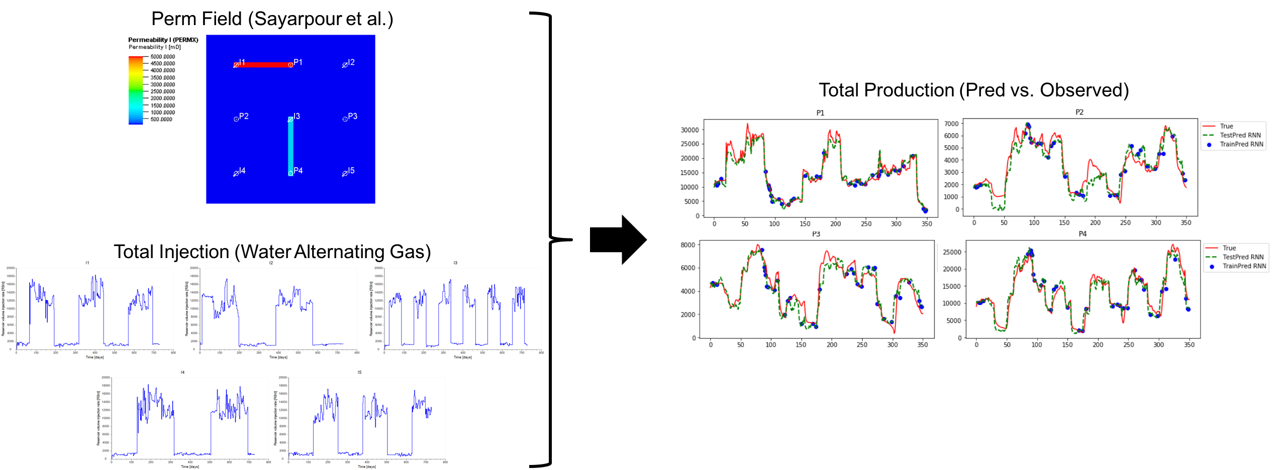
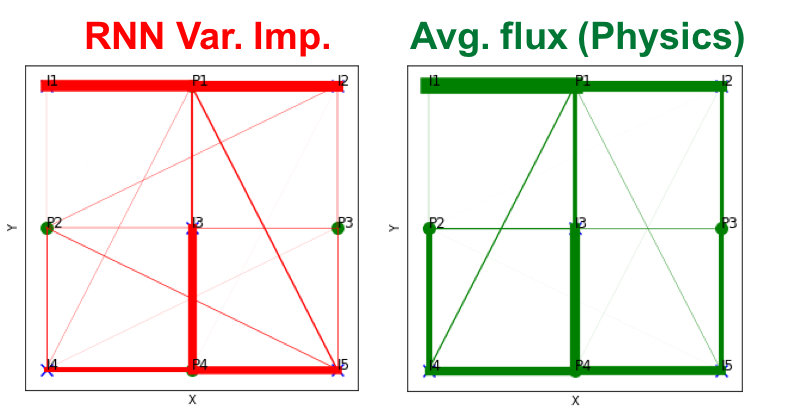
The real value in training an RNN in such a case, would be to infer the connectivity between injectors and producers in the field. This may be measured in terms of the ‘permutation-based variable importance’, where one measures the deviation in the prediction from the true output on shuffling the columns of the inputs. In order to validate such an approach one must clearly define what measure of ‘connectivity’ that is being learned by the RNN. For starters, I compared the average flux from the injectors to producers with the variable importance I computed using the RNN.

Time-Series Clustering Applications to Petrophysics

One of the more established applications of machine-learning in oil and gas would be in the realm of well-log and seismic interpretation. I had the opportunity to work as summer intern with the data science team at TGS-NOPEC, where they specialize in machine-learning applications in the petrophysics/geophysics space. Working with the team was a great learning opportunity for me and I was able to develop an unsupervised approach for anomaly detection in density logs.

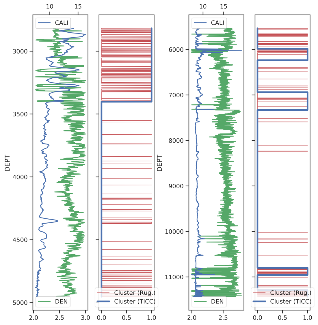
The problem at hand is thus: Wireline density logs measure the rock density in the subsurface at various depths (in the trajectory of the well) by means of gamma-rays (more info here). However, the measurements generally mess up when the tool is not in contact with the formation (rock). Therefore, we need to know the depth intervals at which the tool loses contact with the formation, so that we can delete these portions while pre-processing. Conventionally, this is done by running a caliper log (more info here) along with the density log. This measures the borehole radius in such a way that it mostly remains constant when everything’s going good and shows random fluctuations/increased radius whenever there is a caved-in borehole. Now, this is precisely where the density log fails. Not to mention that this is usually done manually by the petrophysics, for multiple (>300,000 in the Permian) wells!

At TGS, I developed a method that takes as input, a multi-variate time-series (to be accurate, depth series) and does the clustering automatically using an algorithm called Toeplitz Inverse Covariance Clustering (TICC). Turns out, it does the job fairly well (see paper)!

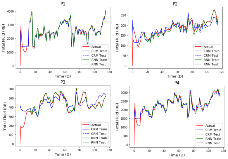
Capacitance-Resistance Models

The capacitance resistance model for inferring interval connectivity was initially developed at UT Austin by Yousef et al (2006). This draws upon the analogy between a reservoir system under pseudosteady state with a resistance-capacitance (RC) circuit. The inputs to the CRM are the injection rates applied at the injectors and the outputs are the production rates at the producer wells. The production rates are computed as a function of the injection rates and several parameters that may be related to the properties of the reservoir system.

Researchers have developed several variations of the CRM model (see here), applicable to specific cases, such as

a. CRM-T(ank)

b. CRM-P(roducer)

c. CRM-I(njector)P(roducer).

As part of a course project (and an initial few months of my PhD), I developed a python implementation of the CRM-P model and did a comparison with recurrent neural network. I applied both to the conventionally used benchmarking case (called the Streak Reservoir). While both models performed fairly well, the RNN model outperformed the CRM model by a marginal degree. The CRM-P code that was used in this comparison has been made publicly available on my github. The RNN code shall be uploaded as soon as our results are published.